
Follow Along with Follow the Winners (NeurIPS 2026)

This post guides you through the high-level ideas of our recent NeurIPS 2026 paper: Follow the Winners: Conservative Policy Improvement with the Cross-Entropy Method for Critic-Free RFT.
At Trent AI we are reimagining the security and robustness of AI Agents. An important part of delivering this vision is specializing agents to meet each customer’s needs. This ranges from the harness around the large language models (LLMs) , such as its orchestration, knowledge and tools, to fine-tuning the model itself. Fine-tuning consolidates domain knowledge and organizational policy into one agent. This often improves both performance and latency compared to longer, more specialized prompts. Although there are many ways to fine-tune LLMs, reinforcement learning fine-tuning (RFT) is especially useful for integrating strategy into the agent.
However, the current RFT toolbox fits our use cases poorly. Group-relative policy optimization (GRPO), one of the most common and successful RFT algorithms, needs several attempts from the same starting point to reduce noise. In many real-world settings, this is unrealistic. Proximal policy optimization (PPO) reduces noise differently, through a second model that predicts the agent’s performance. But this second model adds a lot of overhead, and the costs multiply when we specialize multiple models for many customers.
To see how this becomes a problem, consider an agent that helps investigate a security incident in a live production system. Over many steps, it reads logs and traces what a potential attacker did. We record the whole investigation, but we cannot always rerun it, because a live production system does not stand still. Services get patched and updated, configurations change, and users keep working. A potential attacker could even adapt to our investigation. The world acts of its own accord. For the agent, these changes are unseen variables, so the same investigation can end differently each time. Longer and more complex investigations only add to this noise. Sometimes one wrong turn in a long interaction is enough to send an agent in the wrong direction, giving very different results for similar initial conditions. Our RFT methods must be designed for this setting and operate a constrained budget to keep fine-tuning economically viable. This is where we found GRPO and PPO to fall short.
Our NeurIPS paper proposes an alternative algorithm. Instead of repeated attempts or a second model, our algorithm, Follow the Winners (FTW), keeps a buffer of recent samples and learns to reproduce the better-performing ones. This reduces noise at the cost of slightly higher CPU memory use. We built FTW around a mathematical toolbox called control-as-inference, which puts GRPO, PPO, and FTW side by side in terms of their theoretical objective. This theoretical frame is used to motivate our approximation strategy and prove that our noise-reduction strategy has a controllable noise bias as a result of working strictly with samples.
The remainder of this post walks you through how FTW works mechanically, its assumptions compared to prior methods, and an overview of our results. No math, I promise.
Flow of the Winners
Within the inference toolbox we use, existing optimization methods become straightforward to apply. One of these is the cross-entropy method (CEM) from the late 1990s. The idea is simple. You have something that generates data, you score each item, you keep the best ones, and you update the generator to produce more items like them.
However, a few issues arise when we apply this to LLMs. First, every bit of data is expensive to produce, yet vanilla CEM preserves only a small fraction of data for learning. Second, the scores are noisy and CEM has a harsh cutoff for score filtering. As in the incident example, two similar investigations can score very differently, so a strict filtering cutoff is very likely to preserve too many lucky high scores or throw away good episodes with unlucky low scores. Thus, FTW adapts CEM to mitigate these two issues. First, it keeps episodes from recent versions of the agent in a buffer, so each episode can be reused instead of thrown away. Second, instead of one hard cutoff, it repeatedly draws a small sample from the buffer and keeps the best few items, called the ‘winners’. This gives a softer filter, and we control its strength through the sample size and the number of episodes we keep.
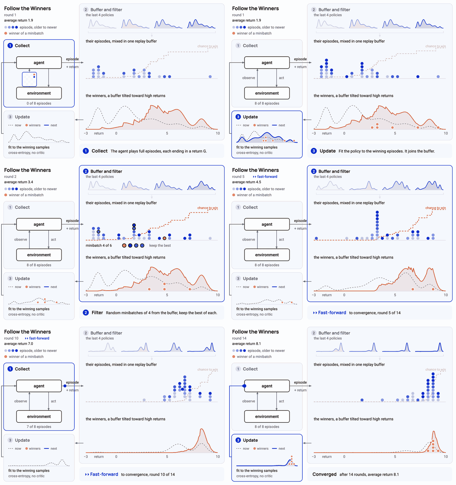
As illustrated in the animation, the core idea of FTW is to start with base weights for an LLM, and then iteratively adjust these base weights based on moving its predictions slowly to desired outputs. This creates a sequence of weights as we let the algorithm run, and we want the final version of this sequence to settle at good performance.
FTW repeats until (near-)convergence the following steps:
- Collect. The current agent with the most recent model weights interacts with the environment. For example, the agent sees a puzzle and says which move to make next, such as ‘go left’. It keeps making moves until the puzzle is solved or time runs out. This sequence of moves is called an episode. Once completed, it is labeled with a score such as 1 if the puzzle was solved and 0 if not, and stored in the data buffer. In the animation these are the blue dots.
- Buffer and filter.
- New completed episodes join the buffer that already holds episodes from the last few versions of the agent. In a first-in-first-out style, the oldest version of the agent gets dropped from the buffer to limit staleness of the data. This is indicated by the blue color gradient in the animation. The curves at the top of step 2 show each agent version’s full distribution, as if it took infinitely many samples.
- The filter re-draws data from the buffer. We draw a small sample, keep its top items for the learning batch, and repeat until the learning batch is full. The learning batch is what we call a tilted version of the buffer, shifted toward the better-scoring episodes. In the animation, this is the orange distribution at the bottom.
- Update. The agent is trained to reproduce this tilted learning batch, so it imitates the better-scoring episodes in the buffer. The update rule is in essence a gradual adjustment from the LLM’s current prediction model to the learning batch. After the update, the agent in step 1 ‘collect’ uses the new weights to gather fresh data.
Over many repetitions, the above steps gradually improve the model weights, eventually settling at good scores (a local optimum). The literal update of the weights toward each round’s filtered winners is what gives our method its name, Follow the Winners.
On a slightly more technical note, our paper also connects the theory of GRPO and FTW. Both algorithms chase a similar target, a version of the agent tilted toward high scores. FTW builds this target directly, much like the statistical bootstrap. It resamples winners from the buffer and imitates them. GRPO instead chases an upper bound of this target. It swaps a soft maximum of the group’s scores for their plain average, so each episode is weighted by how far its score sits from the group average. As a result, GRPO drops the risk-seeking bias from the sample noise that affects FTW. The next section explains what this means concretely.
Do not Follow the Noise
FTW’s risk-seeking bias comes from filtering on the best scores in the buffer. Although a score can be exact, it may still be a noisy measurement of how good an agent’s choice was. The outcome can of course depend on chance or on unseen variables. But even without these, one score covers the whole episode, and the agent’s other moves change from one try to the next. Many good moves can result in a low score because of one bad move later, and a poor move can get lucky. The buffer compounds this. Episodes from older versions of the agent hide how that version chose its moves within the raw data, so for the current update it becomes just another unseen variable. The filter cannot separate this noise from the true average behind each score. So lucky high scores win more often, which pulls FTW away from the best choice on average and toward the noisy one. GRPO is also sensitive to noise, but in a different way. Its target has no risk-seeking bias, but its update rule reacts strongly to noise. In contrast, FTW’s update rule is more conservative and less sensitive to noise, but at the cost of a controllable bias in the target. Fortunately, we can tune it through the sample size we draw from the buffer and how many items from that sample we keep (winners) for the learning batch.
We illustrate this behavior with a concrete example below. We have two choices that an agent can make, and over repeated interactions it needs to find the best choice on average. The catch is that one choice is low-noise and high average, and the other choice is low average, but high noise. This high-noise choice is called the σ-trap.
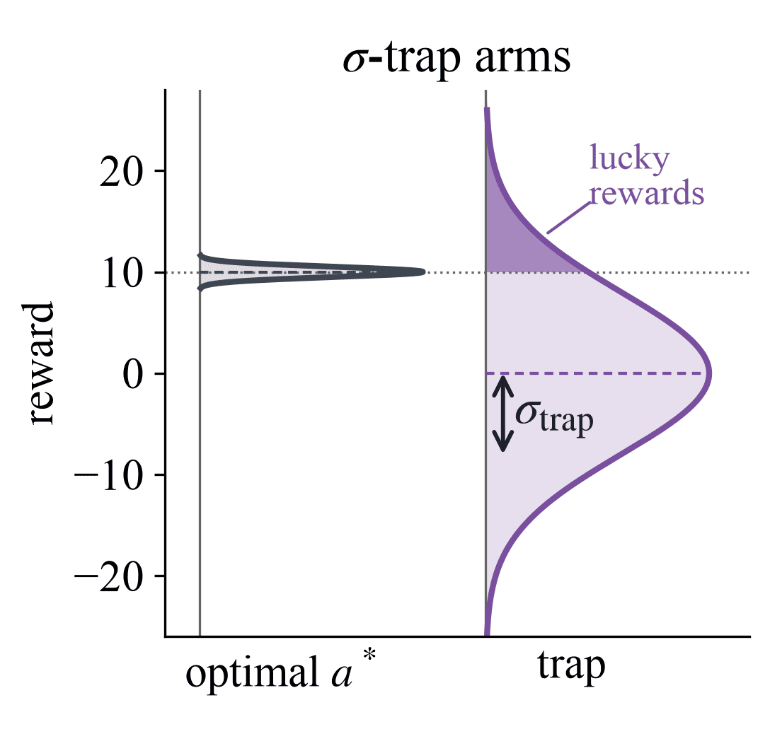

The noisier the trap choice, the more often its lucky episodes land above the optimal choice in terms of score, which then get overrepresented among the winners in the learning batch. The plot on the right shows where each algorithm settles. FTW drifts from the optimal choice a* toward a 50/50 split. GRPO does not seek risk and stays on the optimal choice, but only while its updates remain stable. Eventually, its update rule destabilizes with noise. This is fixable by decreasing GRPO’s step size in the update rule, but this also makes the algorithm very slow. We also see that an extreme version of our algorithm, FTW-exp, which weights items in the buffer exponentially by their score, drowns in the noise very early on.
In the appendix of our paper we show more curves of this risk-seeking bias, which supports our theory that it depends on the two filter settings we mentioned. This is ultimately a fundamental trade-off that we made in getting rid of the second model from PPO, or the repeated attempts that GRPO needs. When we treat all data statically in the buffer we cannot effectively disentangle noise of any form in the scores. Naturally, a more lenient filter lowers the bias but at the cost of slower learning.
Follow the Algorithm Comparison
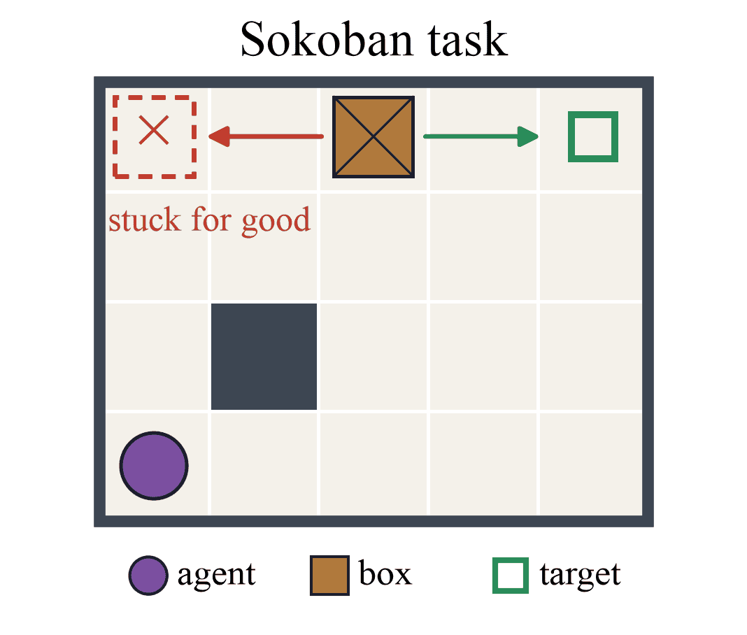
The final part of our paper verifies that our method scales to RFT of LLMs, and that the trade-off against PPO and GRPO is favorable. One of our test environments is Sokoban, a visual puzzle game in which an agent pushes boxes onto targets. We deliberately keep it small, so we can study the algorithm before adding the complexity of, for example, the live incident investigations from our introduction.
The agent plans over multiple steps, and at the end of a full game obtains feedback on whether it solved the puzzle. The agent needs to account for the consequences of its moves, since a single wrong push can prevent successful completion. The left figure below illustrates the task. The right figure shows how each algorithm’s solve rate on unseen puzzles improves during training.
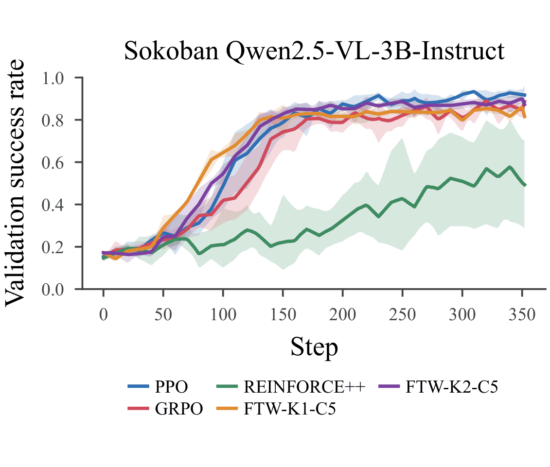
The main takeaway is that FTW matches GRPO and PPO without either of their strict requirements. It needs no repeated attempts from the same start and no second model, only a buffer in CPU memory. To check that the buffer and our filter are what make our method work, we also compare against REINFORCE++. Like FTW, it skips the requirements of both PPO and GRPO, but it replaces them with very little. Instead of GRPO’s average score over repeated attempts, it uses the average score over different attempts in a batch of distinct data. It learns slower and with more noise between runs than FTW.
What Follows
Follow the Winners is the CEM algorithm adapted to LLM agents. It keeps recent episodes in a buffer, filters on small draws from this buffer, and imitates the filtered winners. The buffer and filtering reduce noise and avoid repeated attempts or a second model, which suits agents that operate in dynamic tasks or environments, at the cost of higher CPU memory requirements.
It is not free. Following winners has a risk-seeking bias, which pulls the agent toward lucky outcomes when scores are noisy. Ranking also assumes we can always tell which of two episodes is better, which breaks down in cases like rock-paper-scissors.
On the upside, FTW builds on an imitation learning loss, which makes it easy to extend to, for example, offline datasets. This makes it easier than GRPO to fine-tune on offline and online data together. At Trent AI, for instance, we can seed FTW’s buffer with past incident investigations by our security experts, then let our agent refine that expertise on live incidents. This lets our agents keep improving as new attack strategies arrive. This matters, because live production systems and attackers never stand still.
For more details, read the paper on arXiv and we hope to see you at NeurIPS 2026 in Paris. Our session is scheduled on Thursday, Dec 10 2026, 5:30 PM – 7:30 PM CET. The virtual session is here.